Tutorial

To run the inversion, one need to prepare:

1. Original CMTSource: CMTSource used as starting solution(Ref pycmt3d.source module).
2. Data: including observed data, synthetic data, derived synthetic data and associated windows(Ref pycmt3d.window module)
3. Inversion shema: how to inversion is done(Ref pycmt3d.config module)

1. CMTSource

Pycmt3d needs a source solution as the beginning solution. Source instance could be loaded as:

from pycmt3d.source import CMTSource
cmtfile = "path/to/your/cmtfile"
cmtsource = CMTSource.from_CMTSOLUTION_file(cmtfile)

2. Data

The data that pycmt3d needs includes two part: 1) seismic data; 2) window information associated with the data.

2.1 Window information

The window will provide the window time information. For example, the window file should be formatted like as following:

number_of_total_data_paris
/path/to/observed_data_1
/path/to/synthetic_data_1
number_of_windows_of_pair_1
window_1_begin_time window_1_end_time
window_2_begin_time window_2_end_time
...

A more specific example would be:

2
/home/james/Data/obsd/II.AAK.00.BHZ.sac
/home/james/Data/synt/II.AAK.00.MHZ.sem
3
601.00   712.00
879.00   956.00
1200.00  1421.00
/home/james/Data/obsd/II.ABKT..BHZ.sac
/home/james/Data/synt/II.ABKT..MHZ.sem
1
1600.00 1785.00

If the window file is intended for ASDF, then change the “path/to/file” to station indentification id. The indentification id is specified by “network.station.location.channel”.

2.2 Seismic Data

The data container object could be initialized as:

from pycmt3d.window import DataContainer
from pycmt3d.const import PAR_LIST
npar = 6  # how many perturbed seismograms to be read in
data_con = DataContainer(PAR_LIST[:npar])

Another thing it needs to know is how many number of deriv synthetic files you want to read. The deriv parameter is listed as [Mrr, Mtt, Mpp, Mrt, Mrp, Mtp, depth, longitude, latitude, time shift, hald duration].

If npar is set as 6, then only the first 6 types of perturbed seismograms will be read in, i.e, the seismograms related to the 6 components of moment tensor[Mrr, Mtt, Mpp, Mrt, Mrp, Mtp]. If npar is set as 7, the depth will be added in. If npar is set as 9, then the longitude and latitude will be added in.

If you want to try different Inversion shema, a larger number of npar is preferred. Thus, you can read all necessary deriv synthetic data into the memory and don’t need to load it again.

To really add the data and measurements, there are 2 different methods:

1. sac format data

Then the setup is exactly as the original fortran version. The pycmt3d needs the outputfile from flexwin which contains observed and synthetic data filename and associated windows. Data could be loaded as:

flexwin_file = "path/to/your/flexwin_output"
data_con.add_measurements_from_sac(flexwin_file, tag="user_defined_tag", initial_weight=1.0, load_mode="relative_time")

In this function, tag is user defined tag for the data. For example, if you window selection for two period band, such as 2s-30s and 6s-30s, you can tag the data with “2s-30s” and “6s-30s” ans so they will be treated as two different measurements. Also, you can assign differnt initial_weight to these two categories.

The load_mode is the way how to treat the window time in flexwin file. If load_mode==”relative_time”, then the reference time(zero time point) would be the event time(old version of FLEXWIN). If load_mode==”absolute_time”, then the reference time(zero time point) would be the beginning of the trace. In this case, the window time could not be smaller than 0.

2. ASDF format data

Data could be loaded as:

asdf_file_dict={"obsd":"/path/to/obsd_asdf_file", "synt":"/path/to/synt_asdf_file",
  "Mrr":"/path/to/Mrr_asdf", "Mtt":"/path/to/Mtt_asdf", "Mpp":"/path/to/Mpp_asdf",
  "Mrt":"/path/to/Mrt_asdf", "Mrp":"/path/to/Mrp_asdf", "Mtp":"/path/to/Mrp_asdf"}
flexwin_file = "path/to/your/flexwin_output"
data_con.add_measurements_from_asdf(flexwin_file, asdf_file_dict)

The length of asdf_file_dict should be consistent with napr. If the npar is set as 9, 3 more keys should be added, [“dep”:”/path/to/dep_asdf”, “lon”:”/path/to/lon_asdf”, “lat”:”/path/to/lat_asdf”]

3. Inversion schema

Works partially as the INVERSION.PAR file as the fortran version.

One config example is to 1. invert 9 parameters(moment tensor + depth + location), with location perturbation 0.03 degree, depth perturbation 3.0km and moment perturbation 2.0e23. 2. Weighting will be applied and the no weighting function specified(default weighting function used). 3. Station correction will be applied 4. Constrain includes zero trace but no double couple. 5. Damping set to 0(no damping) 6. Bootstrap will not be used.

Code example as following:

from pycmt3d.config import Config
npar = 9   # 9 paramter inversion
config = Config(npar, dlocation=0.03, ddepth=3.0, dmoment=2.0e+23,
    weight_data=True, weight_function=None, weight_azi_mode="num_files"
    normalize_window=False, norm_mode="data_only", normalize_category=False,
    station_correction=True, zero_trace=True, double_couple=False, lamda_damping=0.0,
    bootstrap=False, bootstrap_repeat=100)

• Bootstrap

  If you want to do some statistic analysis on the inversion, you can turn the bootstrap analysis by turning the bootstrap on by setting “boostrap = True” in the config. It will provide the mean value and the standard deviation. Using this function is encouraged because: 1) it doesn’t cost a lot of extra calculation; 2) give you good estimate how stable is your inversion.

• Window energy normalization

  If you want the measurement from each window normalized by it’s energy, you can set the flag “normalize_window = True” in config. There are two normalization mode you can choose. 1. norm_mode=”data_only” 2. norm_mode=”data_and_synt”(don’t choose this one; bad normalization factor)

• Window Category normalization

  If you want to normalize the measurements from differnt categories, for example, you have window selection from two period bands, 2s-30s and 10s-50s and you want to combine them together in the source inversion, you can turn this flag one to make their contributions equal(all normalize to 1). This flag is usually turned on with window energy normalization on(set both to True).

• Azimuth weighting

  There are two options: 1) “num_files”; 2) “num_wins”. In the old fortran version of cmt3d code, the default is “num_files” and you will use the number of files in each azimuth bin as the weighting term. But you might want to change it to “num_wins” to truely reflect the number of measurements.

4. Source Inversion

After get the CMTSource, Data and Inversion scheme ready, the source inversion can then be conducted:

from pycmt3d.cmt3d import Cmt3D
srcinv = Cmt3D(cmtsource, data, config)
srcinv.source_inversion()

If you want to write out the new synthetic data for the new source and new CMT Solution file:

srcinv.write_new_syn(outputdir="./new_syn")
srcinv.write_new_cmtfile(outputdir=".")

5. Visualization tools

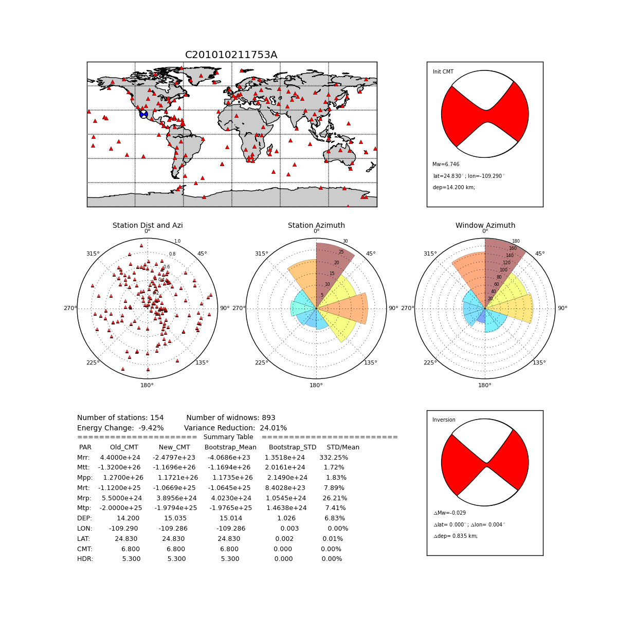
if you want to plot the result of the inversion, use the plotting methods:

srcinv.plot_summary(outputdir=".", format="png")

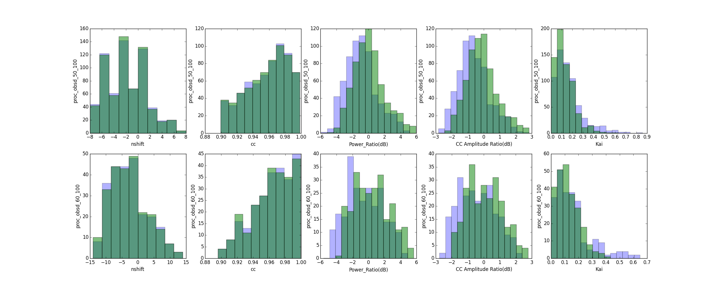
If you want to plot the statistic histogram, for example, how the time shift, energy or waveform misfit(in windows) are changed, you can use:

srcinv.plot_stats_histogram(outputdir=".", format="png")

The format could be any as long as it is supported by matplotlib.

5. Workflow Example

The complete workflow(SAC version) example is shown below:

from pycmt3d.source import CMTSource
from pycmt3d.window import *
from pycmt3d.config import Config
from pycmt3d.cmt3d import Cmt3D
from pycmt3d.const import PAR_LIST

# load cmtsource
cmtfile = "path/to/your/cmtfile"
cmtsource = CMTSource.from_CMTSOLUTION_file(cmtfile)

# load data and window from flexwin output file
npar = 9 # read 9 deriv synthetic
data_con = DataContainer(PAR_LIST[:npar])
flexwin_output = "path/to/your/flexwin_output"
data_con.add_measurements_from_sac(flexwin_output)

# inversion shema
config = Config(npar, dlocation=0.03, ddepth=3.0, dmoment=2.0e+23,
    weight_data=True, weight_function=None, station_correction=True,
    zero_trace=True, double_couple=False, lamda_damping=0.0,
    bootstrap=False)

# source inversion
srcinv = Cmt3D(cmtsource, data, config)
srcinv.source_inversion()

# plot result
srcinv.plot_summary(figurename="/path/to/output_fig")

If it is the ASDF workflow, just replace the data loading part:

# load data and window from flexwin output file
npar = 9 # read 9 deriv synthetic
data_con = DataContainer(PAR_LIST[:npar])
flexwin_output = "path/to/your/flexwin_output"
asdf_file_dict={"obsd":"/path/to/obsd_asdf_file", "synt":"/path/to/synt_asdf_file",
  "Mrr":"/path/to/Mrr_asdf", "Mtt":"/path/to/Mtt_asdf", "Mpp":"/path/to/Mpp_asdf",
  "Mrt":"/path/to/Mrt_asdf", "Mrp":"/path/to/Mrp_asdf", "Mtp":"/path/to/Mrp_asdf",
  "dep":"/path/to/Mrt_asdf", "lon":"/path/to/Mrp_asdf", "lat":"/path/to/Mrp_asdf"}
data_con.add_measurements_from_asdf(flexwin_file, asdf_file_dict)

Other parts would be exactly the same.